 Reproduced, with permission, from:
Kane, S., J. Reilly, and J. Tobey. 1992. An empirical study of the economic effects of climate change on world agriculture. Climatic Change 21: 17-35.
Reproduced, with permission, from:
Kane, S., J. Reilly, and J. Tobey. 1992. An empirical study of the economic effects of climate change on world agriculture. Climatic Change 21: 17-35.
Resources and Technology Division, Economic Research Service, United States Department of Agriculture, 1301 New York Avenue NW, Washington DC 20005-4788, U.S.A.
Abstract. The economic effects of a doubling of atmospheric carbon dioxide concentration on world agriculture under two alternative crop response scenarios are empirically estimated. These effects include both changes in the prices of agricultural commodities as a result of changes in domestic agricultural yields, and changes in economic welfare following altered world patterns of consumption and production of agricultural commodities. Under both scenarios, with a few exceptions, the effects on national economic welfare are found to be quite modest. However, prices of agricultural commodities are estimated to rise considerably under the more pessimistic scenario. Increased agricultural prices reduce consumer surplus and diminish the benefits from climate change that some countries with predicted positive yield effects would otherwise receive.
The economic and social implications of global climate change, due to increases in atmospheric trace gas concentrations, are presently the subject of intense national and international political debate. In order to formulate policies to address this issue, the costs and benefits of the impacts of potential climate change must be identified. The present paper is a preliminary effort to provide some sense of the economic impacts of climate change on world agriculture.
The study of the economic effects of climate change on agriculture is particularly important because agriculture is among the more climate sensitive sectors. However, economic impact assessments of climate change on agriculture are few. Notable exceptions include Adams et al. (1988, 1990) and Arthur (1988). Adams incorporates climate change into a spatial equilibrium model to determine its effects on U.S. agricultural supply and demand. Arthur uses a linear programming model to calculate the effect of climate change on net revenues in the Canadian agricultural sector. and an input/output model to estimate production effects in other sectors of the Canadian provincial economy.
Our paper takes these analyses a step further by examining global, rather than only domestic economic effects. In an open economy, the effect of climate change on agriculture in any individual country cannot be considered in isolation from the rest of the world. Changes in regional climates and agricultural production affect would agricultural prices through international market transactions. Thus, it is not possible to infer the economic effects of climate change on agricultural producers and consumers on the basis of national yield change estimates alone. The important second round impact of changing world agricultural commodity prices on domestic production and consumption must also be captured. Aside from Liverman (1987), who discusses some of the difficulties in applying global food system models to climate change, few researchers have empirically investigated the link between domestic crop yield effects and world agricultural markets.[2]
The paper begins with a brief description of the predictions of large climate models, with a view toward identifying their implications for world agriculture. Because scientific uncertainty is a critical feature of the climate change issue, we make an effort to uncover the shortcomings of these climate change models for the purpose of our analysis. Regional crop yield effects expected to result from broad changes in climate are then examined. Based on our review of yield effects, we impose crop supply shifts in a model of world agriculture to approximate the impact of climate change on selected economic variables.
Climate Predictions
To estimate the agricultural impacts of long-term global climate
changes, we first must have some understanding of the direction and magnitude of climate changes of relevance to agriculture. Climate change projections rely on large, complex computer models, known as General Circulation Models (GCM's). They synthesize our knowledge of the physical and dynamic processes in the overall (atmosphere-ocean-land) climate system, and allow for the complex interactions between the various components. The Intergovernmental panel on Climate Change (IPCC), composed of hundreds of scientists worldwide, recently released a scientific assessment of climate change. Based on current model results the IPCC (1990) predicts[3]:
(1) Global mean surface warming as greenhouse gases partially block or absorb heat radiating from the earth. The rate of increase of global mean temperature is predicted to be about 0.3[[ring]]C per decade. This will result in a likely increase in global mean temperature of about 3[[ring]]C before the end of the next century.(2) Regional climate changes different from the global mean. Models predict that surface air will warm faster over land than over oceans and that the warming is expected to be 50-100% greater than the global mean in high northern latitudes in winter. Temperature increase in Southern Europe and central North America are also predicted to be higher than the global mean.
(3) Increased precipitation in the order of 5-10% in middle and high latitude continents (35-55[[ring]]N) in winter. Reduced summer precipitation and soil moisture in Southern Europe and Central North America.
(4) An average rate of global mean sea level rise of about 6 cm per decade over the next century mainly due to thermal expansion of the oceans and the melting of some land ice. A sea level rise of about 65 cm is predicted by the end of the next century.
Features of Climate Models and implications for Agriculture
There are several limitations associated with the use of GCM predictions for agricultural impact studies. We have identified three areas of concern. They include timing. geographical scale of predictions, and seasonality.
Timing. Climate models have, for the most part, been developed to project the equilibrium state of climatic conditions under an effective doubling of carbon dioxide concentrations in the atmosphere. Typically, they do not provide information on the dynamic time path to the new equilibrium climate. The timing of the climate effects are dependent upon estimates of future greenhouse gas emissions and physical lags between changes in trace gas concentrations and climate effects. Calculating greenhouse gas concentrations in the atmosphere many decades in the future is inherently difficult. For example, interactions between physical sources and sinks and changes in climate are not fully understood; nor is the contribution of many economic activities to the total level of trace gas emissions.
Climate fluctuations during the transition period to the equilibrium state could also have important economic consequences. Even though it is generally presumed that the long-run temperature trend will be a fairly persistent increase with year-to-year variations, the transient response of temperature change to increased trace gas concentrations is not well understood and may not be linear.
Geographical Scale. Currently, GCM's agree strongly in direction for many globally averaged phenomenon, the best example of which is surface air temperature. However on regional scales, there are significant differences. The difference in some estimates of temperature changes for the U.S. midwest is more than 3[[ring]]C in the summer season (Grotch, 1989). The grid size of the GCM's determines the level of detail of predictions. Currently the smallest grid size of GCM's is in the order of 250,000 km[2], too large for reliable regional and local impact assessments.
Poor regional resolution also limits researchers' ability to predict changes in soil moisture levels, a critical element in determining plant growth potential, and thus agricultural impacts. Soil moisture levels are dictated by precipitation which is a localized climate feature, and consequently not well simulated by GCM's.
Seasonality. GCM's have only a limited capability to project seasonality; that is, the difference between average summer and winter temperatures. Seasonality is an important determinant of crop production systems. Changes in precipitation and temperature would have very different effects on crop production depending on their seasonal distribution.
Climate Effects across Broad Geographic Zones
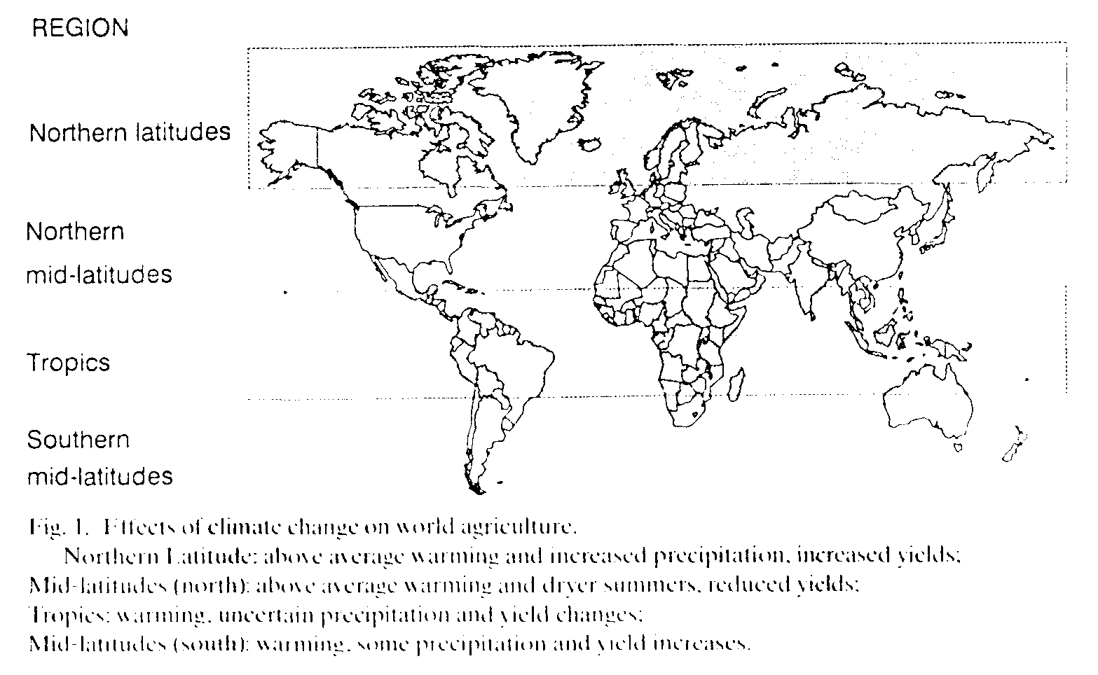
Although GCM predictions are not ideal for agricultural impact analysis, they serve as a suitable benchmark for our global economic analysis directed at evaluating general directions and relative magnitudes of change. In particular, the GCM predictions suggest broad geographical zones across which climate change may affect agriculture (see Figure 1). Increased precipitation and warming in the high northern latitudes could enhance agricultural production potential in the northern regions of the Soviet Union, Canada, and Europe.
Drying in the interior of continents in the northern middle latitudes combined with warming could lead to negative crop and livestock effects in the nited States and Western Europe, and the most agriculturally productive regions of Canada. This region includes the largest grain producing areas of the world. Other northern middle latitude regions, including southeast Asia, could suffer from coastal inundation.
There are exceptions to the broadly generalized climate patterns sketched by the IPCC. While China falls within the category of northern middle latitude countries, climate models do not strongly support increased aridity. Consequently, some estimates suggest crop production potential could increase (Zhang, 1989).
Regions of agricultural importance in the southern middle latitudes include Argentina and Australia. The climate change effects on agriculture in Argentina are not well known. However, some projections show a wetter, and therefore more agriculturally productive climate for the major agricultural regions in Australia (IPCC, 1990; Walker et al., 1989).
Much less is known about the possible agricultural effects of climate change in the tropical latitudes encompassing regions of Africa, Latin America, and Southeast Asia. In general, temperature changes are expected to be smaller in equatorial regions than in higher latitudes, but there is very little agreement on changes in precipitation and soil moisture. Consequently, both magnitude and direction of effects on agriculture are uncertain. We observe, however, that less severe temperature changes may not necessarily result in less severe agricultural effects. Evapotranspiration increases nonlinearly with temperature. Thus, the potential for drought with a one degree rise in temperature in areas with already high average temperatures is greater than in cooler areas. In addition, cooler temperate areas may be able to shift to warm weather grains, whereas already warm areas may have fewer immediate alternatives.
Crop Growth Models
The broad changes in climate projected by GCM's offer some guidance for assessing agricultural effects, but they must be complemented with more detailed information in order to evaluate region-specific effects on crop growth. Mathematical crop growth models are used to translate modified weather conditions into crop yield changes by simulating plant growth rates for a particular crop, combining information on physical conditions (sunlight, temperature, rainfall, and soil type) with growth processes.
Many types of crop-weather models have been used in agricultural impact studies, including empirical/statistical, simulation, and extrapolation from historical record. Predictions from these models must be interpreted carefully in light of the manifold problems that exist. Limitations of crop-weather models include the following: multicollinearity among predictor variables; non-linearity between precipitation, yield, and temperature; noncompatibility of spatial scale between data on climate and agricultural yield; limited time-scale of data sets that preclude capturing changes in soil characteristics such as content and soil erosion; and, the use of historical data that frequently do not include extreme events that may result from climate change (see Katz, 1979; Santer, 1985; Liverman, 1987; and Arthur, 1988).
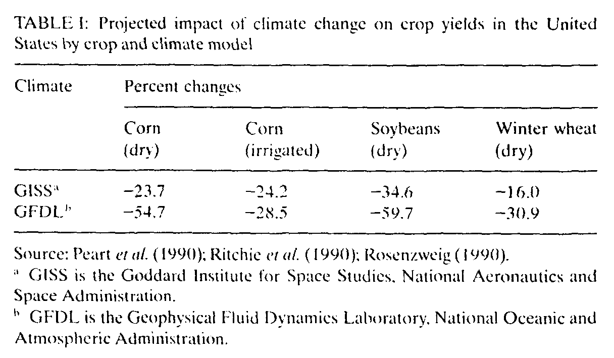
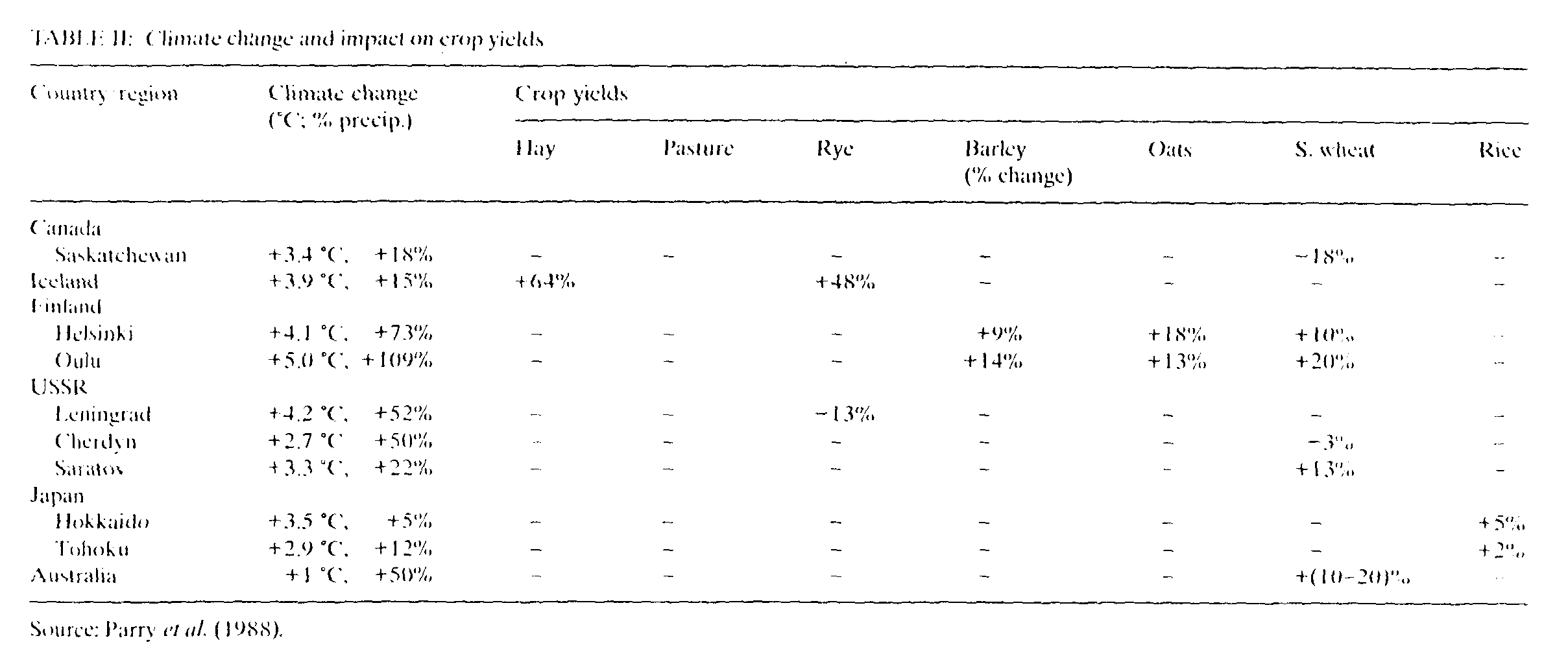
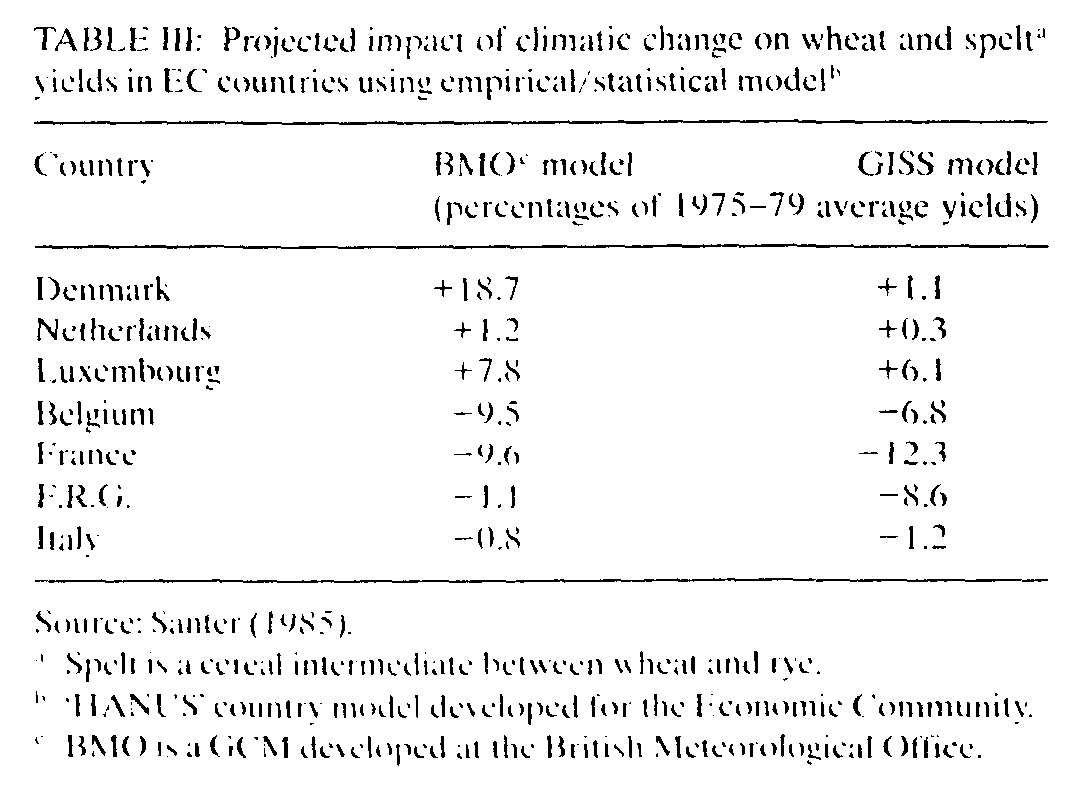
We review a number of yield estimates found in the literature on the crop growth impacts of climate change, including USEPA (1990), Parry et al. (1988), and Santer (1985). While not a comprehensive global assessment, these studies have examined a wide range of region-specific changes in yields induced by changes in climate as suggested by GCMs, under existing cropping patterns, management practices, and production technologies. A selective summary of the results of these studies is shown in Tables I, II, and III. Even though each producing area was examined by a different team of experts using different models and methods of analysis, the findings of these studies generally support the conclusion that middle latitude yields will fall and northern latitude yields will rise with a doubling of CO2 levels.
Santer found modest positive effects on crop yields in northern areas in Europe, and modest negative effects in southern European areas. parry and others examined the effect of climate variation on agriculture in semi-arid regions in Ecuador, Brazil, Kenya, India, Australia, and the USSR, and northern latitude agriculture in Canada, sub-Arctic USSR, Finland, Japan, and Iceland. In general, the effects of predicted climate change were positive on northern latitude agriculture where production is currently limited by short growing seasons and cool temperatures. In Iceland, yields of hay were estimated to increase by 64%. In Finland, barley yields were estimated to increase 9 to 14% in the south. Spring wheat and oat yields were estimated to increase by 10 to 20, and 13 to 18%, respectively. In the northern regions of the USSR examined in the study, rye yields and spring wheat were estimated to decrease by 13 and 3% due to excessive soil moisture.
In the semi-arid regions examined by Parry and others, estimates for a doubling of CO2 were made for wheat in Canada, the USSR, and Australia. Both the USSR and Australia showed increased yields due largely to the predicted increase in precipitation. Canada, however, showed decreased yields of spring wheat of 18% due to the adverse effects of increased temperature and reduced soil moisture.
The USEPA study compared the agricultural effects of predicted climate chance under effective CO2 doubling based on two different climate model forecasts. Both the Goddard Institute for Space Studies (GISS) and Geophysical Fluid Dynamics Laboratory (GFDL) climate models predict warming and drying for most agricultural areas of the United States. The GFDL model predicts more severe warming and drying with heightened effects during the summer growing season. Yield declines in the range of 16 to 35deg.% are reported under the GISS climate prediction, and yield declines in the range of 25 to 60% are found under the GFDL climate predictions.
Other Considerations
In addition to temperature and precipitation changes, climate change may also impact agriculture through greater competition from weeds, increased plant and animal disease, changes in soil nutrients and pests, and increased conflicts for available water. While these damaging effects are probably controllable, we are far from concluding what they may do the cost of agricultural production and how they will affect agricultural resources and the environment.
They are, however, probably less important than the impact that increased carbon in the atmosphere may have on plant growth. A carbon enriched atmosphere, like that under doubled CO2 concentrations, is widely believed to promote plant growth and also lead to increased efficiency in water use. This positive influence of climate change on plant growth is termed the CO2 fertilization effect. To date, there are no reliable estimates of its precise magnitude; existing 'chamber' studies of plant growth test separately for the effects of controlled climatic conditions and varying levels of carbon in the atmosphere.
Despite the limits of scientific knowledge, some crop response studies have attempted to take into account both altered climatic conditions, and the direct effect of climate change on plant growth. Their analyses suggest that the increase in yields from enhanced carbon levels could be significant. Parry et al. (1988) found that in sub-Arctic regions of the USSR, inclusion of the CO2 fertilization effect increased yields 17%. The USEPA (1990) study found that inclusion of the positive effects of CO2 on plant growth generally balanced yield reductions in the GFDL scenarios[4], and resulted in modest to large increases under the GISS scenario. Finally, a recent study conducted by the National Climate Program Office (NCPO, 1989) concluded that, under the assumption that no other factors are limiting, the fertilization effect from an effective doubling of carbon dioxide concentration, could be expected to enhance crop yields by about 15%. Beyond this point, or with carbon dioxide levels in excess of 600 ppm, most of the benefits of the direct effect on plant growth are exhausted.
The Model Structure
The GCM climate models and crop response studies serve as the basis for our analysis of the economic effects of climate change on agriculture. Their suggested crop effects are introduced into a world food model - the Static World Policy Simulation (SWOPSIM) modeling framework. SWOPSIM describes world agricultural markets through a system of domestic supply and demand equations that are specified by matrices of variables that describe the responsiveness of the quantity of agricultural commodities supplied and demanded to changes in commodity prices (i.e., own and cross price elasticities). It is a primary tool for policy analysis of international agricultural markets, developed by the Economic Research Service, United States Department of Agriculture, Descriptions of the SWOPSIM model can be found in Krissoff et al.(1990), Roningen (1986), and Roningen and Dixit (1989).
SWOPSIM has the desirable feature of encompassing all regions of the world at a considerable degree of commodity disaggregation. The model contains 20 agricultural commodities, including eight crop, four meat/livestock, four dairy product, two protein meal, and tow oil product categories. SWOPSIM is flexible enough to allow separate identification of up to 36 countries/regions of the world. For the purposes of this study we decomposed the world into 13 countries/regions including the United States, Canada, the European Community (EC), Australia, Argentina, Pakistan, Thailand, China, Brazil, the USSR, other Europe (Sweden, Finland, Norway, Austria, and Switzerland), and Japan. All other countries are grouped together. This level of disaggregation covers the major agricultural importing and exporting regions of the world and several areas projected to be among the most strongly affected by climate change.
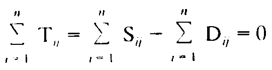
The model's structure is straightforward.[5] For each country/region i and commodity j (or k) in the model, a demand and supply function is specified:
Dij = Dij(CPij,CPik)
Sij = Sij(PPij, PPik)
where CPij and PPij are domestic prices facing consumers and producers of commodity j. CPik is the cross-product consumer price for commodity k (that is, the consumer price of other commodities that affect the demand for j); PPik is the price of an intermediate input to product j, and/or the price of another product that affects the price of commodity j. Trade is the difference between domestic supply and demand:
Tij = Sij - Dij.
Domestic prices depend on the level of consumer and producer support wedges (SCWij and PSWij) and world prices denominated in local currency:
CPij = CSWif + F(Ei * WPj),
PPij = PSWij + G(Ei * WPj),
where CSWij and PSWij are measures of the level of government supporting each country, as measured by Producer and Consumer Subsidy Equivalents (PSEs/CSEs).
The PSE/CSE is a broader measure of policy support than the nominal rate of protection (see Webb et al., 1990). It includes direct income payment, input, marketing, and structural assistance as well as market price support. Ei is the exchange rate defined as local currency (i) dollar and WPi is the world price of commodity j.
World markets clear when net trade of a commodity across all countries is equal to 0. For commodity j, this occurs when world supply of a commodity equals its world demand:
The commodity supply and demand equations are parameterized to reproduce 1986 base period data for each countries' supply, demand, prices, and trade. The data set is published in Sullivan et al. (1989). When a change is introduced to the model, world trade, production, consumption, and prices, are rebalanced. The pattern of prices and quantities observed in the base period is then compared to the pattern that emerges from the model.
Replication of base period data is not, in itself, evidence that the model is valid. Rather, validity is determined by the reasonableness of the properties of the model. An important property of considerable interest is the measure of producer and consumer response to price changes. In an assessment of the validity of the SWOPSIM model. Roningen and Dixit (1989) find that the parameters used in the model to estimate these responses (the aggregate supply and demand elasticities) are consistent with the literature, including the models used in OECD (1987) and Parikh et al. (1988). The responsiveness of commodity trade to changes in prices is also derived. This is the partial net trade elasticity. They tested this responsiveness for the United States largely because of the availability of such information for comparative purposes. Again, they found that the net trade elasticities compare favorably with empirical estimate provided by the literature.
The SWOPSIM modeling framework has some desirable characteristics for our purposes. Among these is its ability to estimate the welfare effects of agricultural production disturbances. In contrast, most empirical models of agriculture ignore traditional welfare and resource efficiency measures (some widely used agricultural models in this category include FAPSIM (Gadson et al., 1982), WHEATSIM (Holland and Sharples, 1981), FAPRI (Meyers et al., 1986), and POLYSIM (Ray and Richardson, 1978)). Welfare effects are measured by the change in consumer and producer surplus. Consumer and producer surplus are commonly in consumer and producer surplus. consumer and producer surplus are commonly used empirical measures of how much better, or worse off, consumers or producers are when commodity prices are altered. Consumer surplus is defined as the area under the demand curve and above the price line. It represents a willingness to pay beyond what is actually paid. Producer surplus is defined as the area below the price line and above the supply curve. It measures the excess of gross receipts over total variable costs.[6]
SWOPSIM also has some limitations that should be noted. First, it is a partial-equilibrium model and does not capture agricultural interactions with other economic sectors. However, we do not believe that this is a serious limitation. In industrialized and semi-industrialized countries, agricultural production is only a small part of total output and therefore has relatively little effect on resource allocations in other sectors. Moreover, in a general equilibrium study of climate change in the United States, Kokoski and Smith (1987) show that the welfare effects of fairly large, single-sector imparts, can be adequately measured in a partial-equilibrium setting.
Second, the SWOPSIM modeling framework does not explicitly incorporate resource inputs. Rather, the model implicitly assumes that uses of resource supplies, including arable land, will be appropriately altered to fulfill new demand and supply conditions following a shock to the base system. It would be useful to have resource inputs in the model in order to exogenously change them and to ensure that, for large shocks to the system, constraints on resources (especially cultivated area) are not binding.
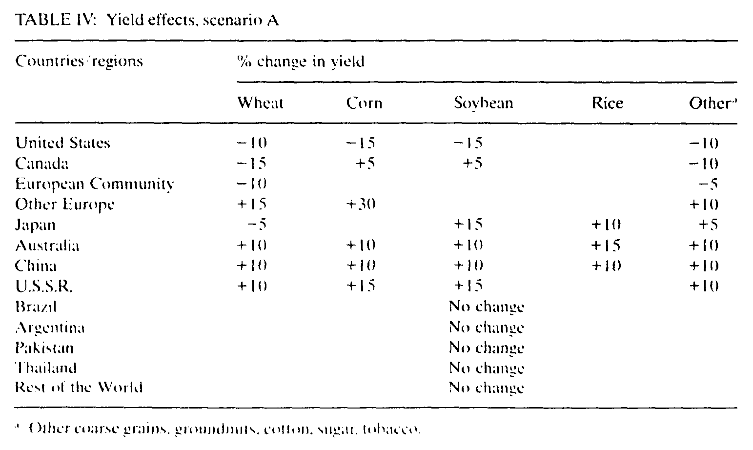
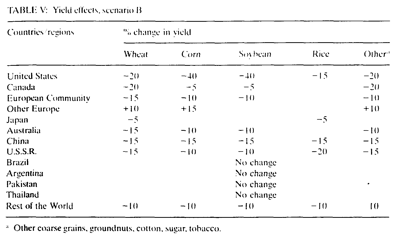
Two Scenarios
The SWOPSIM modeling framework does not include explicit climate variables. Climate changes are introduced as exogenous increases or decreases in base yields for specific countries/regions. Once entered into SWOPSIM, the model then solves for a new set of consumption, production, and price relationships. Two alternative climate change scenarios, termed 'A' and 'B' are specified (see Table IV and V). They should not be viewed as 'upper' and 'lower' bounds to potential outcomes, but rather as outcomes that illustrate the range of possibilities (of a doubling of CO2 levels) suggested by the existing literature. Scenario A reflects moderate impacts and Scenario B reflects very adverse impacts. The scenarios were used in some of the preliminary research undertaken by the IPCC Working Group 2 on Impacts (see Parry 1990). Scenario A yield effects are close to the estimates provided by Parry et al. (1988) and Santer (1985). We have not assumed any CO2 fertilization effects. Farmer responses to climate changes are also not included For these reasons the assumed yield changes are more likely to overstate than understate the actual changes
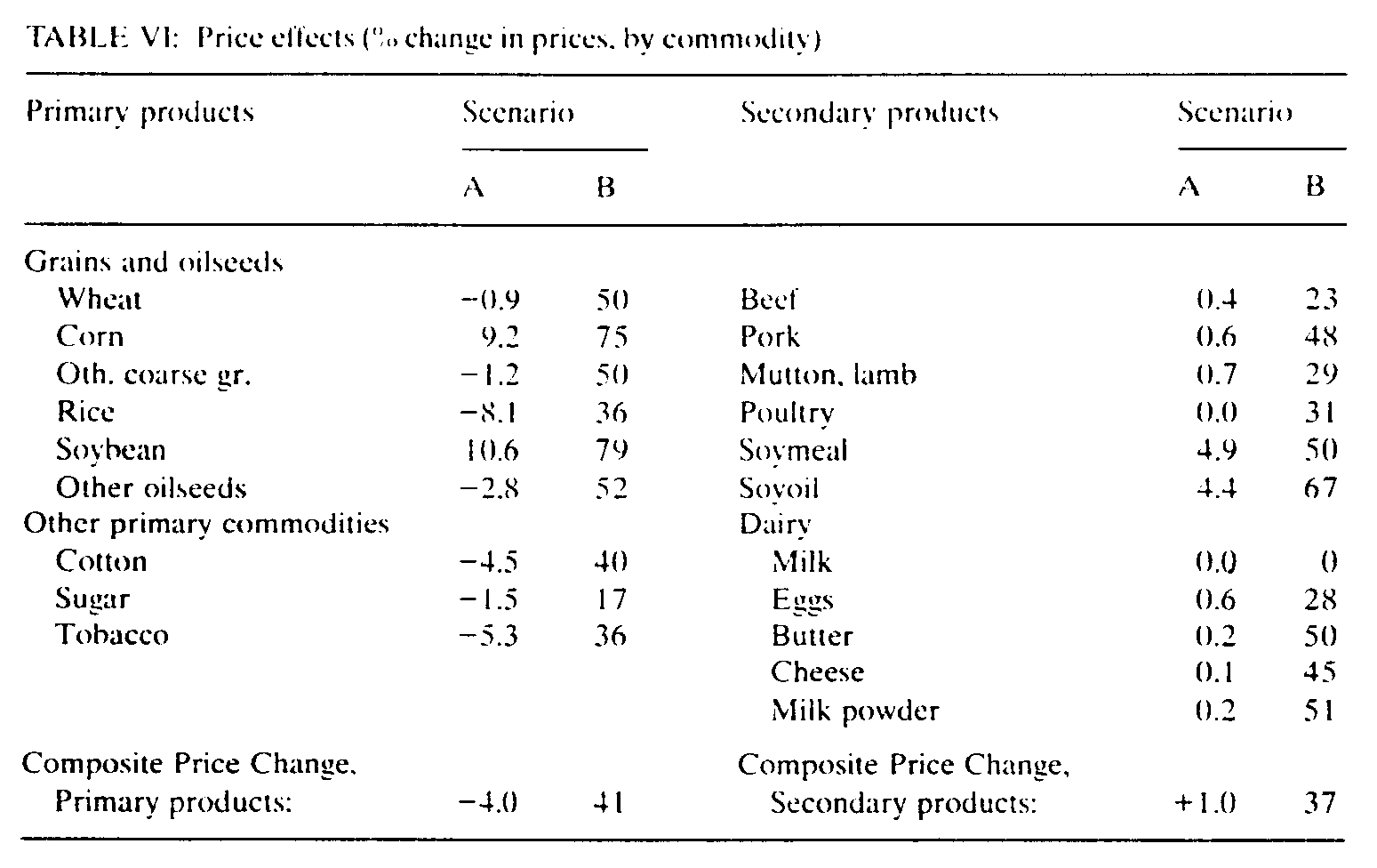
Price and Income Effects
The estimated price effects of these crop yield changes generated by SWOPSIM are presented in Table VI. Under scenario A, compared to the base, there is a predicted small decline in the price of primary products, and a small increase in the price of secondary products. This result is not surprising since most corn and soybean production occurs in countries located in regions of the world that are expected to be adversely affected by climate change. Of the secondary agricultural products, oil and meal prices increase by the highest percentage, reflecting their dependence on soybeans and other oilseed intermediate inputs.
In contrast, scenario B predicts large increases in the world price of primary and secondary agricultural products - 41 and 37% respectively. These large price increases are directly related to the much more pessimistic yield effects, particularly in those countries that are the most important producers. In corn and soybeans, the change in U.S. yields from base is -15% in scenario A, and 440% in scenario B. Because the United States accounted for 43 and 56% of world corn and soybean production in 1986 (measured in total tonnage: USDA 1989), such a large change in yield effects can be expected to have a considerable effect on world agricultural prices. Similarly, the largest producer of rice is China (36.6% of world production). The change in Chinese yields from base is +15 and -15% in scenarios A and B respectively. The largest producers of wheat are the USSR, China, and the United States. They accounted for 17.2, 16.7, and 10.6% of 1986 world production. The change in their wheat yields from base is +10 to -15 for the USSR and China, and -10 to -20 for the United States.
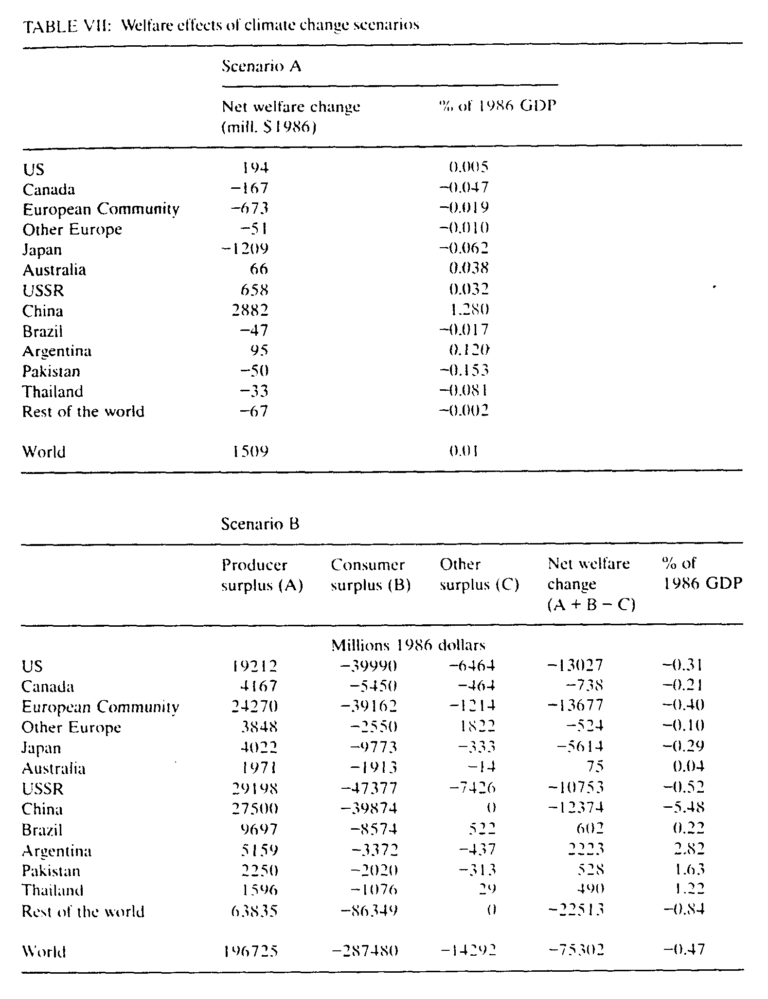
Table VII presents the complete breakdown of estimated changes in consumer and producer surplus for scenario B, as well as the change in taxpayer costs ('other surplus') when there are distortions in agricultural markets form government intervention. For scenario A, only the net welfare change is presented.
The results in Table VII illustrate two interesting features regarding the impact of climate change on agriculture. First, even under the assumption of relatively large and negative domestic yield effects, the economic impacts on national economies are estimated to be small, with some winners and some losers. The new world welfare effect is negative but very modest even under the more pessimistic scenario B; it is estimated to be 0.47% of 1986 world gross domestic product (GDP). Aside from China, no country/region is predicted to experience welfare losses greater than one percent of GDP. The relatively small macro-economic impact of climate change on domestic economies is related to the fact that agriculture accounts for only a small percent of GDP in most economies (3 percent in industrial market economies, and 19% in developing economies in 1986; World Bank, 1988).
Second, the pattern of welfare effects among countries depends not only on domestic yield changes, but also on changes in world commodity prices, and the relative strength of the country as a net agricultural importer or exporter. Consider scenario B. Aside from 'other Europe', all countries/regions are predicted to experience negative yield effects from climate change. However, in every case the change in producer surplus is positive. This is due to the fact that reduced domestic yields from climate change increase international agricultural prices, and higher producer prices increase producer surplus. In contrast, with demand curves unchanged, the same price effect reduces consumer surplus.
The importance of induced price changes in promoting interregional adjustments in production and consumption can be illustrated by comparing the SWOP-SIM results with other models that consider the climate change effects on a single country. Adams et al. (1988) examine the economic impact of climate change on U.S. agriculture using the GISS and GFDL climate models. They find net welfare reductions for the United States under the two scenarios to be about $7 and $34 billion ($ 1982) respectively. Referring back to Table I, IV, and V, we notice that the EPA (1990) crop yield effects in the United States under the GISS and GFDL climate models roughly resemble our U.S. yield changes specified in Scenario A and B. However, we find that the welfare changes for the United States are +$0.2 and -$13 billion (1986$) for scenario A and B, respectively. These values are considerably smaller than the Adams et al. predictions. We interpret the differences as an indication of the role of international price changes in promoting interregional adjustments in production and consumption.[7]
The net welfare effect of climate change on domestic economies depends critically on a country's net trade position. The producer surplus gain will be large relative to the consumer surplus loss if the country is a large net exporter. For example, although Australia is predicted to experience significant yield losses under scenario B. the net consumer plus producer surplus effect is positive. In this case, because Australia is a very large net exporter, the rise in world agricultural prices generates a large increase in producer surplus that dominates the yield decline losses, and the loss in consumer surplus associated with a higher price of agricultural commodities. In contrast, Japan is a large net importer with losses in consumer surplus very large relative to producer surplus gains.
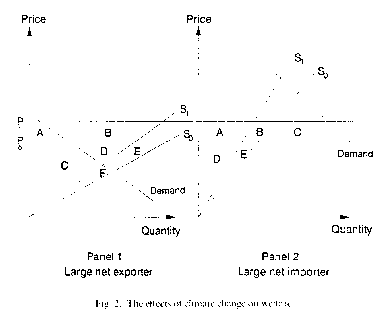
These two possibilities are shown diagrammatically in Figure 2. Consistent with scenario B results, we assume that equilibrium would agricultural prices rise (from P0 to P1) and domestic agricultural yields fall, shifting aggregate supply curves (from S0 to S1). Panel 1 represents the case of a large net exporter (at world prices, quantity supplied is greater than quantity demanded). The loss in consumer surplus is given by the area 'A;--the area under the demand curve between the old and new price. The gain in producer surplus is give by (A+B) - (E+F)- the area above the old supply curve between the old and new price, less the area under the old price that is lost when the supply curve shifts inward. Straightforward algebra tells us that if area 'B' is greater than the area (E+F), there is a net gain in consumer plus producer surplus. Panel 2 represents the case of a large net importer. The loss in consumer surplus is given by the area (A+B+C). The gain in producer surplus is given by (A-E). Thus, if (B+C) is greater than 'E', there is a net loss in consumer plus producer surplus.
Climate change is a severe test of our economic modeling capability. Imperfect knowledge about long-term climate changes, physical crop growth changes, and changes in critical economic conditions, make empirical economic estimations of the agricultural impacts of climate change informed speculation at best.
Our world agricultural model is static in the sense that it does not assume any farm responses to changing climatic conditions, and does not introduce changes in technology, population, or other growth conditions. Thus, the empirical results provide a 'snapshot' of the economic effects that a doubling of CO2 levels might have on world agriculture, given present agricultural technologies, structure of production, and demand conditions. They should not be interpreted as accurate representations of the agricultural consequences of climate change on specific economies. Rather, they highlight general directions and the order of magnitude of change, as well as demonstrating some straightforward, but important economic principles.
Future empirical applications of the model could be aimed at uncovering the implications of other economic changes to the system. We do not suggest that credible growth predictions can be made. But, as Sonka and Lamb (1987) observe, sensitivity analysis would be useful to better understand the interrelations of a changing climate with a dynamic economic system.
Although climate change presents researchers with a very difficult modeling problem, we feel that impact assessments such as this are useful inputs in policy-making when used carefully. In particular, a central argument to our analysis is that the evaluation of climate change winners and losers cannot be made on the basis of domestic yield effects alone. The impacts of climate change on agriculture must be analyzed globally, taking account of regional differences in the impacts, and the role of price changes in promoting interregional adjustments in production and consumption, Thus, policymakers' perception of the structure of incentives to reduce greenhouse gas emissions should not be based solely on predicted national agricultural production changes, but rather on how these yield effects alter global agricultural markets, and consequently, domestic producer and consume welfare.
5 This description follows Krissof et al. (1990).
Adams, R., McCar, B., Dudek, D., and Glyer,J.: 1988, 'Implications of Global Climate Change for Western Agriculture', Western J.Agric. Econ. 12(2), 348-356.
Adams, R., Rosenzweig, C., Peart, R., Ritchie,J., McCar.,R., Glyer, J.,Curry, R., Jones, J., Boote, K., and Allen, Jr., L.: 1990 'Global Climate Change and U.S. Agriculture', Nature 345(17), 219-223.
Arthur, L.: 1988, 'The Greenhouse Effect and the Canadian Prairies', in Johnston,G., Freshwater, D., and Favero, P., (eds.), Natural Resource and Environmental Policy Issues, Westview Press, Inc., Boulder.
Gadson, K., Price, J., and Salathe, L.,: 1982, 'Food and Agricultural Policy Simulator (FAPSIM): Structurla Equations and Variable Definitions', ERS STaff Report No. AGES820506, U.S. Department of Agriculture, May 1982.
Grotch, S.: 1989, 'Regional Intercomaprison of General Circulation Model Predictions and Historical Climate Data', U.S. Department of Energy, Office ofEnergy Research. DOE/NBB/0084. Washington, D.C.
Haley, S. and Dixit, P.: 1988, 'Economic Welfare Analysis: An Application to the SWOPSIM Modeling Framework', ERS Staff Report Number AGES87125. U.S. Department of Agriculture, Washington.
Holland, F. and Sharples, J.: 1981, 'WHEATSIM: Model 15 Description and Computer Program Documentation', Station bulletin No. 319, Purdue Univeristy, March 1981.
Intergovernmental Panel on Climate Change: 1990, Climate Change: The IPCC Scientific Assessement, Cambridge University Press, Cambridge.
Katz, R.: 1979, 'Climate Model Simulations of the Equilibrium Climatic Response to Increaed Carbon Dioxide', Rev. Geophys. 25, 760-798.
Kokoski, M. and Smith. V.: 1987, 'A General equilibrium Analysis of Partial-Equilibrium Welfare Measures, The Case of Climate change', Amer. Econ. Rev: 77, 331-341.
Krissoff, B., Sullivan, J., and Wainio, J.: 1990, 'Developing Countries in an Open Economic: The Case of AGricultural Trade', in Glodin I. and Knudsen, O. (eds.), Agricultural Trade Liberlization, Organization for Economic Cooperation and Development, Paris, France.
Liverman, D.: 1987, 'Forecasting the Impact of Climate on Food Systems: Model Testing and Model Linkage', Climatic Change 11, 267-285.
Meyers, W., Devadoss, S., and Helmar, M.: 1986, Baseline Projections, Yield Impacts and Trade Liberalization Impacts for Soybeans, Wehat, and Feed Grains: A FAPRI Trade Model Analysis'. Working Paper No. 86-WP2. The Center for Agricultural and Rural Development, University of Iowa.
National Climate Program Office: 1989, 'Climate Impact Response Functions,' Report of thecoolfront Wrokshop, West Virginia. September 11-14, 1989.
National Research Council: 1987, Current Issues in Atmospheric Change, National Academy Press. Washington.
Organization for Economic Cooperation and Development: 1987, National Policies and Agricultural Trade, Paris, France.
Parikh, K., Fischer, G., Frohberg, K., and Gulbrandsen, O.: 1988. Towards Free Trade in Agriculture. Martinus Nijhoff Publishers, Dordrecht.
Parry, M., Carter,T., and Konijn, N. (eds.): 1988, The Impact of Climatic Variations on Agriculture. Volume 1: Assessments in Cool Temperate and Cold Regions, HASA UNEP,and Volume 2: Assesments in Semi-Arid Regions, HASA/UNEP, Kluwer Academic Publishers, Boston.
Parry, M.: 1990, Climate Change and World Agriculture, London, Earthscan Publications Limited.
Peart, R., Jones, J., and Curry, R.: 1990,'Impact of Climate Change on Crop yield in the Southeastern U.S.A.', in The Potential Effects of Global Climate Change on the United States, Report to Congress, Volume 3, Washington, D.C.
Ray, D. and Richardson, J.: 1978, 'Detailed Descriptions of POLYSIM', Technical Bulletin T-151, Agricultural Experiment Station, Oklahoma State University, December 1978.
Ritchie, J., Gaer, B., and Chou, T.: 1990, 'Effect of Global Climate Change on Agriculture: Great Lakes Region', in The Potential Effects of Global Climate Change on the United States, Report to Congress, Volume 3, Washington, D.C.
Roningen, V.: 1986, 'A Static World Policy Simulation (SWOPSIM) Modeling Framework', ERS Staff Reprot AGE860625, U.S. Department of Agriculture, Washington.
Roningen, V. and Dixit, P.: 1989, 'How Level is the Playing Field?', Foreign Agricultural Economic Report Number 239, Economic Research Service, U.S. Department of Agriculture, Washington.
Rosenzweig, C.: 1990, 'Potential Effects of Climate Change on Agricultural Production in the Great Plains: A Simulation Study', in The Potential Effects of Global Climate Change on the United States. Report to Congress, Volume 3, Washington, D.C.
Santer, B.: 1985,'The Use of General Circulation Models in Climate Impact Analyses - A Preliminary Study of the Impacts of a CO2 Induced Climate Change on West European AGriculture', Climatic Change 7, 71-93.
Sonka, S. and Lamb, P.: 1987, 'On Climate Change and Economic Analysis', Climatic Change 11, 291-311.
Sullivan, J., Wainio, J., and Roningen, V.: 1989, 'A Database for Trade Liberalization Studies', ERS Staff Report Number AGES89-12, U.S. Department of Agriculture, Washington.
USDA: 1989, 'World Agricultural Trends and Indicators, 1970-88.' ERS Statistical Bulletin Number 781, U.S. Department of Agriculture, Washington.
USEPA: 1990, The Potential Effects of Global Climate Change on the United States, Volume 103. Report to Congress, U.S. Environmental Protection Agnecy, Washington, D.c.
Walker, B., Young, M., Parslow, J., Crocks, K., Fleming, P., Margules, C., and Landsberg, J.: 1989, 'Global Climate Change and Australia: Effects on Renewable Natural Resources'. CSIRP Divison of Wildlife and Ecology, Canberra, Australia.
Webb, A., Lopez, M., and Penn, R.: 1990, 'Estimates of Producer and Consumer Subsidy Euivalents', ERS Statistical Bulletin Number 803. U.S. Department of Agriculture, Washington.
Willig, R.: 1976, 'Consumer Surplus without Apology', Amer. Econ.Rev. 66, 589-97.
World Bank: 1988, World Development Report 1988, Oxofrd University Press, New York.
Zhang, J.: 1989, 'The CO2 Problem in Climate and Dryness in North China', Meterol. Monthly 15, 308.
(Received 6 August, 1990; in revised form 31 July, 1991)